A Retrieval-Augmented Generation (RAG) chatbot for the Ahmedabad Municipal Corporation’s sanitation services, built using Streamlit, LangChain, and Mixtral-8x7B.
Overview
This project implements an AI-powered chatbot that answers questions about sanitation policies for the Ahmedabad Municipal Corporation (AMC). The bot uses RAG architecture to provide accurate, context-aware responses based on official documentation.
Features
Interactive chat interface using Streamlit
RAG implementation using LangChain
Document processing with PyMuPDF
Vector storage using Pinecone
Mixtral-8x7B language model integration
Automatic bullet-point formatting for long responses
Technical Stack
Frontend: Streamlit
Language Model: Mixtral-8x7B-Instruct-v0.1
Vector Database: Pinecone
Embeddings: HuggingFace Embeddings
Document Processing: PyMuPDF
Framework: LangChain
Setup
Clone the repository:
git clone https://github.com/sleeky-glitch/sanitationbotamc.git
cd sanitationbotamc
Install dependencies:
pip install -r requirements.txt
Set up environment variables:
Create a .env file with the following:
Etcd v3.1.0 or greater is required.   To use the v3 API make sure to set environment
variable ETCDCTL_API=3.  Precompiled binaries can be downloaded at https://github.com/etcd-io/etcd/releases.

$etcd = Net::Etcd->new(); # host: 127.0.0.1 port: 2379
$etcd = Net::Etcd->new({ host => $host, port => $port, ssl => 1 });

# put key
$put_key = $etcd->put({ key =>'foo1', value => 'bar' });

# check for success of a transaction
$put_key->is_success;

# get single key
$key = $etcd->range({ key =>'test0' });

# return single key value or the first in a list.
$key->get_value

# get range of keys
$range = $etcd->range({ key =>'test0', range_end => 'test100' });

# return array { key => value } pairs from range request.
my @users = $range->all

# delete single key
$etcd->deleterange({ key => 'test0' });

# watch key range, streaming.
$watch = $etcd->watch( { key => 'foo', range_end => 'fop'}, sub {
    my ($result) =  @_;
    print STDERR Dumper($result);
})->create;

# create/grant 20 second lease
$etcd->lease( { ID => 7587821338341002662, TTL => 20 } )->grant;

# attach lease to put
$etcd->put( { key => 'foo2', value => 'bar2', lease => 7587821338341002662 } );

# add new user
$etcd->user( { name => 'samba', password => 'foo' } )->add;

# add new user role
$role = $etcd->role( { name => 'myrole' } )->add;

# grant read permission for the foo key to myrole
$etcd->role_perm( { name => 'myrole', key => 'foo', permType => 'READWRITE' } )->grant;

# grant role
$etcd->user_role( { user => 'samba', role => 'myrole' } )->grant;

# defrag member's backend database
$defrag = $etcd->maintenance()->defragment;
print "Defrag request complete!" if $defrag->is_success;

# member version
$v = $etcd->version;

# list members
$etcd->member()->list;
DESCRIPTION
Net::Etcd is object oriented interface to the v3 REST API provided by the etcd grpc-gateway.
ACCESSORS
host
The etcd host. Defaults to 127.0.0.1
port
Default 2379.
name
Username for authentication, defaults to $ENV{ETCD_CLIENT_USERNAME}
password
Authentication credentials, defaults to $ENV{ETCD_CLIENT_PASSWORD}
ca_file
Path to ca_file, defaults to $ENV{ETCD_CLIENT_CA_FILE}
key_file
Path to key_file, defaults to $ENV{ETCD_CLIENT_KEY_FILE}
cert_file
Path to cert_file, defaults to $ENV{ETCD_CLIENT_CERT_FILE}
cacert
Path to cacert, defaults to $ENV{ETCD_CLIENT_CACERT_FILE}.
The token that is passed during authentication. This is generated during the
authentication process and stored until no longer valid or username is changed.
The etcd v3 API is in heavy development and can change at anytime please see api_reference_v3
for latest details.
Authentication provided by this module will only work with etcd v3.3.0+
LICENSE AND COPYRIGHT
Copyright 2018 Sam Batschelet (hexfusion).
This program is free software; you can redistribute it and/or modify it
under the terms of either: the GNU General Public License as published
by the Free Software Foundation; or the Artistic License.
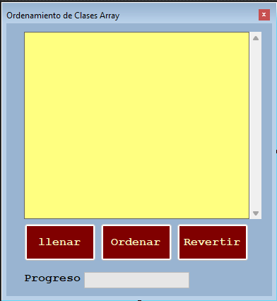
Este proyecto hace el llenado de un TextBox con Arreglos numericos
de manera aleatoria con la funcion Rnd( ), Adicionalmente se trabaja
con una Barra de Progreso que mostrara la carga de cada elemento del
arreglo en el textbox. Tambien se emplearan los Metodos Ordenar ()
y Revertir() para luego volver a cargar todo el arreglo en pantalla.
Descripcion
Se hace la siguiente declaracion del Arreglo: Dim RandArray(0 To 2999)
As Long. Posteriormente se definen los limites superior e inferior
de la Barra de Progreso que mostrara la carga de todos los elementos del
Arreglo en el TextBox. Despues se recorre y rellena el Arreglo Numerico
conn la funcion Rnd() con numeros Aleatorios tipo Long. Y en ese orden
aleatorio apareceran en el cuadro de texto. Se llama a la funcion
Array.Sort a traves de la siguiente instruccion: Array.Sort(RandArray)
Este proyecto ordenara todo el arreglo al hacer clic en el correspondiente
boton recorriendo luego todo el arreglo y mostrandolo por pantalla en
el TextBox y la Barra de Progreso mostrara el avance de la carga del
Arreglo. el mismo proceso ocurrira con el metodo Array.Reverte para
invertir el orden del arreglo a traves de la siguiente instruccion:
Array.Reverse(RandArray).
Actualizacion: 08/01/2025
Hora: 07:13
Detalles técnicos del proyecto:
Idioma: Visual Basic.NET
Versión del framework: 4.7.2
Array Class Sorting
This project fills a TextBox with random numeric arrays using the Rnd() function.
Additionally, a Progress Bar is used to show the loading of each element
of the array in the textbox. The Sort() and Reverse() methods will also be used to
reload the entire array on the screen.
Description
The following Array declaration is made: Dim RandArray(0 To 2999) As Long.
The upper and lower limits of the Progress Bar are then defined to show
the loading of all the elements of the Array in the TextBox. Then the Numeric Array
is traversed and filled using the Rnd() function with random Long-type numbers.
And in that random order they will appear in the text box. The Array.Sort function
is called through the following instruction: Array.Sort(RandArray).
This project will sort the entire array by clicking on the corresponding
button, then going through the entire array and displaying it on the screen in
the TextBox and the Progress Bar will show the progress of the array loading.
The same process will occur with the Array.Reverte method to reverse the order of the
array through the following instruction:
Array.Reverse(RandArray).
Update: 01/08/2025
Time: 07:13
Technical details of the project:
Language: Visual Basic.NET
Framework version: 4.7.2
Code of the Project:
Public Class Form1
Dim RandArray(0 To 2999) As Long
'Abre el objeto barra de progreso y muestra el numero de elementos
Private Sub Form1_Load(sender As Object, e As EventArgs) Handles MyBase.Load
    ProgressBar1.Minimum = 0
    ProgressBar1.Maximum = UBound(RandArray)
    Label2.Text = UBound(RandArray) + 1

End Sub

Private Sub btnllenar_Click(sender As Object, e As EventArgs) Handles btnllenar.Click
    'Completa el arreglo con numeros aleatorios, y los despliega en un cuadro de texto
    Dim i As Integer

    For i = 0 To UBound(RandArray) 'Ubond: Funcion que devuelve el indice superior de un Arreglo
        RandArray(i) = Int(Rnd() * 1000000)
        txtOrder.Text = txtOrder.Text & RandArray(i) & vbCrLf
        ProgressBar1.Value = i 'hacer que avance la barra de progreso
    Next i
End Sub

Private Sub btnOrdenar_Click(sender As Object, e As EventArgs) Handles btnOrdenar.Click
    'Ordena el arreglo mediante el metodo Array.Sort
    Dim i As Integer
    txtOrder.Text = ""
    Array.Sort(RandArray)

    For i = 0 To UBound(RandArray) 'Ubond: Funcion que devuelve el indice superior de un Arreglo
        txtOrder.Text = txtOrder.Text & RandArray(i) & vbCrLf
        ProgressBar1.Value = i 'mueve la barra de avance
    Next i
End Sub

Private Sub btnRevertir_Click(sender As Object, e As EventArgs) Handles btnRevertir.Click
    'Revierte de los elementos del arreglo, utilizando Array.Reverse
    Dim i As Integer
    txtOrder.Text = ""
    Array.Reverse(RandArray)

    For i = 0 To UBound(RandArray) 'Ubond: Funcion que devuelve el indice superior de un Arreglo
        txtOrder.Text = txtOrder.Text & RandArray(i) & vbCrLf
        ProgressBar1.Value = i 'hacer que avance la barra de progreso
    Next i
End Sub
For many automated perception and decision tasks, state-of-the-art
performance may be obtained by algorithms that are too complex for
their behavior to be completely understandable or predictable by human
users, e.g., because they employ large machine learning models.
To integrate these algorithms into safety-critical decision and control
systems, it is particularly important to develop methods that can
promote trust into their decisions and help explore their failure modes.
In this article, we combine the anchors methodology
[1]
with Monte Carlo Tree Search (MCTS) to provide local model-agnostic explanations
for the behaviors of a given black-box model making decisions by
processing time-varying input signals.Our approach searches for highly descriptive explanations for these
decisions in the form of properties of the input signals, expressed in
Signal Temporal Logic (STL), which are highly likely to reproduce the
observed behavior.
To illustrate the methodology, we apply it in simulations to the
analysis of a hybrid (continuous-discrete) control system and a
collision avoidance system for unmanned aircraft (ACAS Xu) implemented
by a neural network.
Basic definitions
Let $f: X \rightarrow \lbrace 0, 1 \rbrace$ be a black-box model and
$x_0 \in X$ be a given input instance for which we want to explain the model’s
output $f(x_0)$.
anchor
An anchor is defined as a rule $A_{x_0}$ verified by $x_0$ whose precision
(see below) is above a certain threshold $\tau \in [0, 1]$.
It can be viewed as a logic formula describing via a set of rules (predicates)
a neighborhood $A_{x_0} \subset X$ of $x_0$, such that inputs
sampled from $A_{x_0}$ lead to the same output $f(x_0)$ with high probability.
precision
The precision of a rule $A$ is the probability that the black-box model’s
output is the same for a random input $z$ satisfying $A$ as for $x_0$:
$$\text{precision}(A) := \mathbb P(f(z) = f(x_0) \, | \, z \in A)$$
coverage
The coverage of a rule $A$ is the probability that a random input satisfies $A$:
$$\text{coverage}(A) := \mathbb P(z \in A)$$
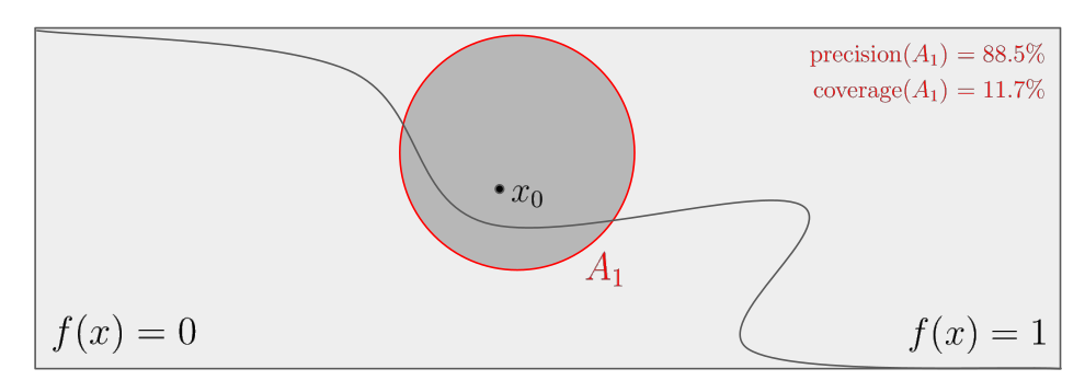
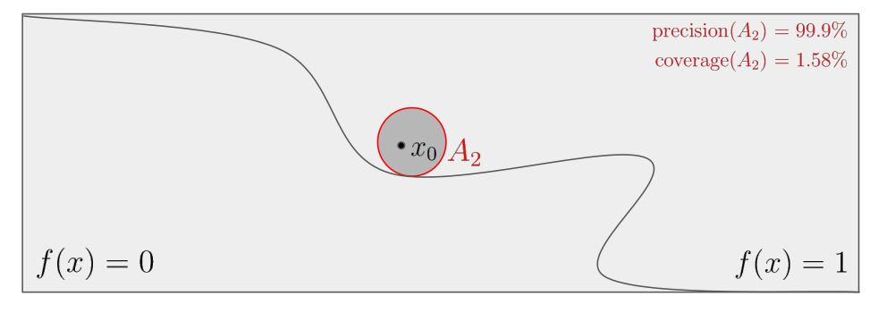
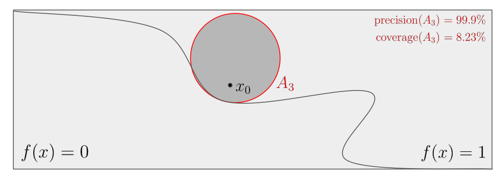
Illustration
The figure below illustrates the notions of precision and coverage.
On this figure, the curved boundary separates the decision $f(x) = 1$ from the
other $f(x) = 0$.
Suppose that the threshold $\tau$ defining an anchor is fixed at 99%.
Then $A_1$ is not a valid anchor because of its low
precision, but $A_2$ and $A_3$ are. Finally, $A_3$ is preferred to $A_2$
because of its higher coverage.
Although only the precision is involved to define anchors, rules that have
broader coverage, i.e., that are satisfied by more input instances, are
intuitively preferable.
Essentially, an explanation of high precision approximates an accurate
sufficient condition on the input features such that the output remains the
same, while a larger coverage makes the explanation more general, thus
approaching a necessary condition.
Therefore, [1]
proposes to maximize the coverage among all anchors to find
the best explanations, i.e., among those which have sufficient precision.
This anchor with maximized coverage allows to locally approximate the boundary
separating the inputs leading to the specific output $f(x_0)$ from the rest.
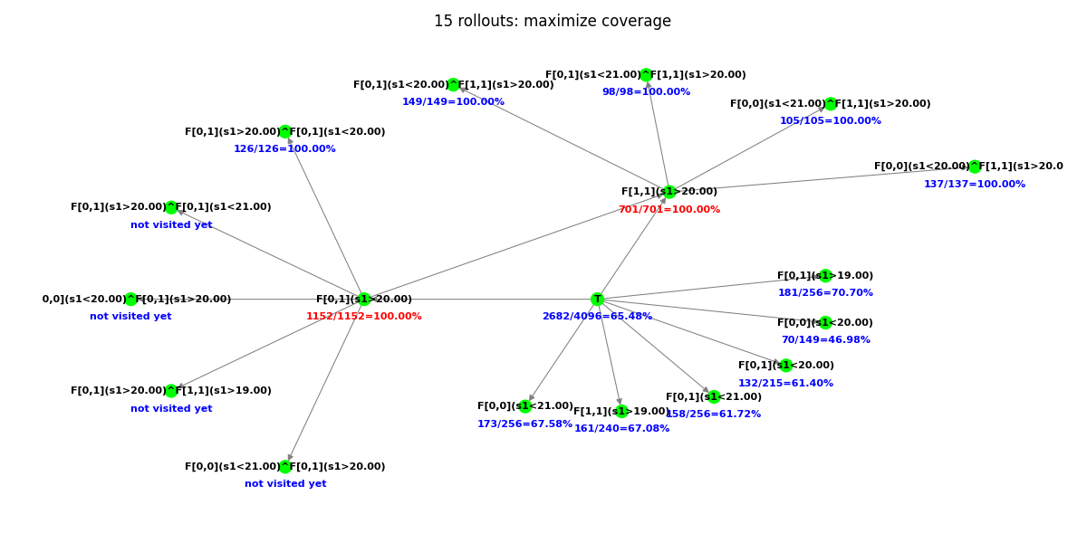
Thermostat: an illustrative example
We provide a simple example to illustrate the evolution of a Directed Acyclic
Graph (DAG) built with the proposed MCTS algorithm.
We work here over the discrete time set $t \in \lbrace 0, 1 \rbrace$.
Consider an automated thermostat, measuring the temperature signal
$s_1(t)$ of a room at times $t = 0$ (the reference time) and $t = 1$.
At time $t = 1$, it switches off if at least one of the values $s_1(0)$,
$s_1(1)$ is greater than 20°C.
Suppose that this mechanism is unknown to us but that we can perform
simulations of this thermostat.
Consider a measured signal [19°C, 21°C].
We observe that the thermostat switches off at t = 1 for this signal,
and we seek to provide an explanation for this behavior.
We use first-level primitives, with the parameter $\mu$ allowed to take the values 19°C, 20°C, 21°C.
Starting from the trivial STL formula $\top$, we perform 15 roll-outs
and show in the following the construction (the first snapshots) of the DAG,
necessary to identify the next move from $\top$.
At the end, the algorithm returns $\mathbf{F}_{[0,1]}(s_1 > 20^{\circ}\text{C})$
with its 100% empirical precision.
In words, this explanation says:
“the thermostat is switched off at t = 1 because the temperature
is above 20°C at least once in the interval $\mathbf{[0, 1]}$“,
which corresponds exactly in this case to how the thermostat indeed works.
Repository organization
 |- main.py      - Main executable script
 |- mcts.py      - Tree object implementing MCTS steps
 |- stl.py       - STL objects (primitives & formulas)
 |- visual.py    - Script for visualization of the tree evolution (Section 4.3)
 |- simulator.py - Abstract class for simulators
 |
 |  **folders**
 |- simulators   - Simulators that can generate signal samples (function `simulate`)
 |- demo         - Figures and important log files
 |_ log          - Automatically generated log files
Usage
The code was developped in Python 3.8 and should only require basic packages
such as numpy.
In main.py, multiple case studies (see here
for details) can be run successively by uncommenting the corresponding lines:
defmain(log_to_file: bool=False) ->None:
"Run algorithm in multiple case studies."set_logger() # log to terminalsimulators= []
simulators.append('thermostat')
#simulators.append('auto_trans_alarm1')#simulators.append('auto_trans_alarm2')#simulators.append('auto_trans_alarm3')#simulators.append('auto_trans_alarm4')#simulators.append('auto_trans_alarm5')#simulators.append('auto_trans')#simulators.append('acas_xu')forsimulatorinsimulators:
iflog_to_file:
set_logger(simulator)
run(simulator)
The argument --log [-l] logs the (intermediate & final)
results to a log folder:
python3 main.py [--log [-l]]
For the automated thermostat specifically, the evolution of the DAG shown above
can be visualized with visual.py:
python3 visual.py
Acknowledgements
This work was funded by NSERC
under grant ALLRP 548464-19.
For many automated perception and decision tasks, state-of-the-art
performance may be obtained by algorithms that are too complex for
their behavior to be completely understandable or predictable by human
users, e.g., because they employ large machine learning models.
To integrate these algorithms into safety-critical decision and control
systems, it is particularly important to develop methods that can
promote trust into their decisions and help explore their failure modes.
In this article, we combine the anchors methodology
[1]
with Monte Carlo Tree Search (MCTS) to provide local model-agnostic explanations
for the behaviors of a given black-box model making decisions by
processing time-varying input signals.Our approach searches for highly descriptive explanations for these
decisions in the form of properties of the input signals, expressed in
Signal Temporal Logic (STL), which are highly likely to reproduce the
observed behavior.
To illustrate the methodology, we apply it in simulations to the
analysis of a hybrid (continuous-discrete) control system and a
collision avoidance system for unmanned aircraft (ACAS Xu) implemented
by a neural network.
Basic definitions
Let $f: X \rightarrow \lbrace 0, 1 \rbrace$ be a black-box model and
$x_0 \in X$ be a given input instance for which we want to explain the model’s
output $f(x_0)$.
anchor
An anchor is defined as a rule $A_{x_0}$ verified by $x_0$ whose precision
(see below) is above a certain threshold $\tau \in [0, 1]$.
It can be viewed as a logic formula describing via a set of rules (predicates)
a neighborhood $A_{x_0} \subset X$ of $x_0$, such that inputs
sampled from $A_{x_0}$ lead to the same output $f(x_0)$ with high probability.
precision
The precision of a rule $A$ is the probability that the black-box model’s
output is the same for a random input $z$ satisfying $A$ as for $x_0$:
$$\text{precision}(A) := \mathbb P(f(z) = f(x_0) \, | \, z \in A)$$
coverage
The coverage of a rule $A$ is the probability that a random input satisfies $A$:
$$\text{coverage}(A) := \mathbb P(z \in A)$$
Illustration
The figure below illustrates the notions of precision and coverage.
On this figure, the curved boundary separates the decision $f(x) = 1$ from the
other $f(x) = 0$.
Suppose that the threshold $\tau$ defining an anchor is fixed at 99%.
Then $A_1$ is not a valid anchor because of its low
precision, but $A_2$ and $A_3$ are. Finally, $A_3$ is preferred to $A_2$
because of its higher coverage.
Although only the precision is involved to define anchors, rules that have
broader coverage, i.e., that are satisfied by more input instances, are
intuitively preferable.
Essentially, an explanation of high precision approximates an accurate
sufficient condition on the input features such that the output remains the
same, while a larger coverage makes the explanation more general, thus
approaching a necessary condition.
Therefore, [1]
proposes to maximize the coverage among all anchors to find
the best explanations, i.e., among those which have sufficient precision.
This anchor with maximized coverage allows to locally approximate the boundary
separating the inputs leading to the specific output $f(x_0)$ from the rest.
Thermostat: an illustrative example
We provide a simple example to illustrate the evolution of a Directed Acyclic
Graph (DAG) built with the proposed MCTS algorithm.
We work here over the discrete time set $t \in \lbrace 0, 1 \rbrace$.
Consider an automated thermostat, measuring the temperature signal
$s_1(t)$ of a room at times $t = 0$ (the reference time) and $t = 1$.
At time $t = 1$, it switches off if at least one of the values $s_1(0)$,
$s_1(1)$ is greater than 20°C.
Suppose that this mechanism is unknown to us but that we can perform
simulations of this thermostat.
Consider a measured signal [19°C, 21°C].
We observe that the thermostat switches off at t = 1 for this signal,
and we seek to provide an explanation for this behavior.
We use first-level primitives, with the parameter $\mu$ allowed to take the values 19°C, 20°C, 21°C.
Starting from the trivial STL formula $\top$, we perform 15 roll-outs
and show in the following the construction (the first snapshots) of the DAG,
necessary to identify the next move from $\top$.
At the end, the algorithm returns $\mathbf{F}_{[0,1]}(s_1 > 20^{\circ}\text{C})$
with its 100% empirical precision.
In words, this explanation says:
“the thermostat is switched off at t = 1 because the temperature
is above 20°C at least once in the interval $\mathbf{[0, 1]}$“,
which corresponds exactly in this case to how the thermostat indeed works.
Repository organization
 |- main.py      - Main executable script
 |- mcts.py      - Tree object implementing MCTS steps
 |- stl.py       - STL objects (primitives & formulas)
 |- visual.py    - Script for visualization of the tree evolution (Section 4.3)
 |- simulator.py - Abstract class for simulators
 |
 |  **folders**
 |- simulators   - Simulators that can generate signal samples (function `simulate`)
 |- demo         - Figures and important log files
 |_ log          - Automatically generated log files
Usage
The code was developped in Python 3.8 and should only require basic packages
such as numpy.
In main.py, multiple case studies (see here
for details) can be run successively by uncommenting the corresponding lines:
defmain(log_to_file: bool=False) ->None:
"Run algorithm in multiple case studies."set_logger() # log to terminalsimulators= []
simulators.append('thermostat')
#simulators.append('auto_trans_alarm1')#simulators.append('auto_trans_alarm2')#simulators.append('auto_trans_alarm3')#simulators.append('auto_trans_alarm4')#simulators.append('auto_trans_alarm5')#simulators.append('auto_trans')#simulators.append('acas_xu')forsimulatorinsimulators:
iflog_to_file:
set_logger(simulator)
run(simulator)
The argument --log [-l] logs the (intermediate & final)
results to a log folder:
python3 main.py [--log [-l]]
For the automated thermostat specifically, the evolution of the DAG shown above
can be visualized with visual.py:
python3 visual.py
Acknowledgements
This work was funded by NSERC
under grant ALLRP 548464-19.
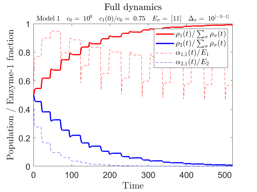
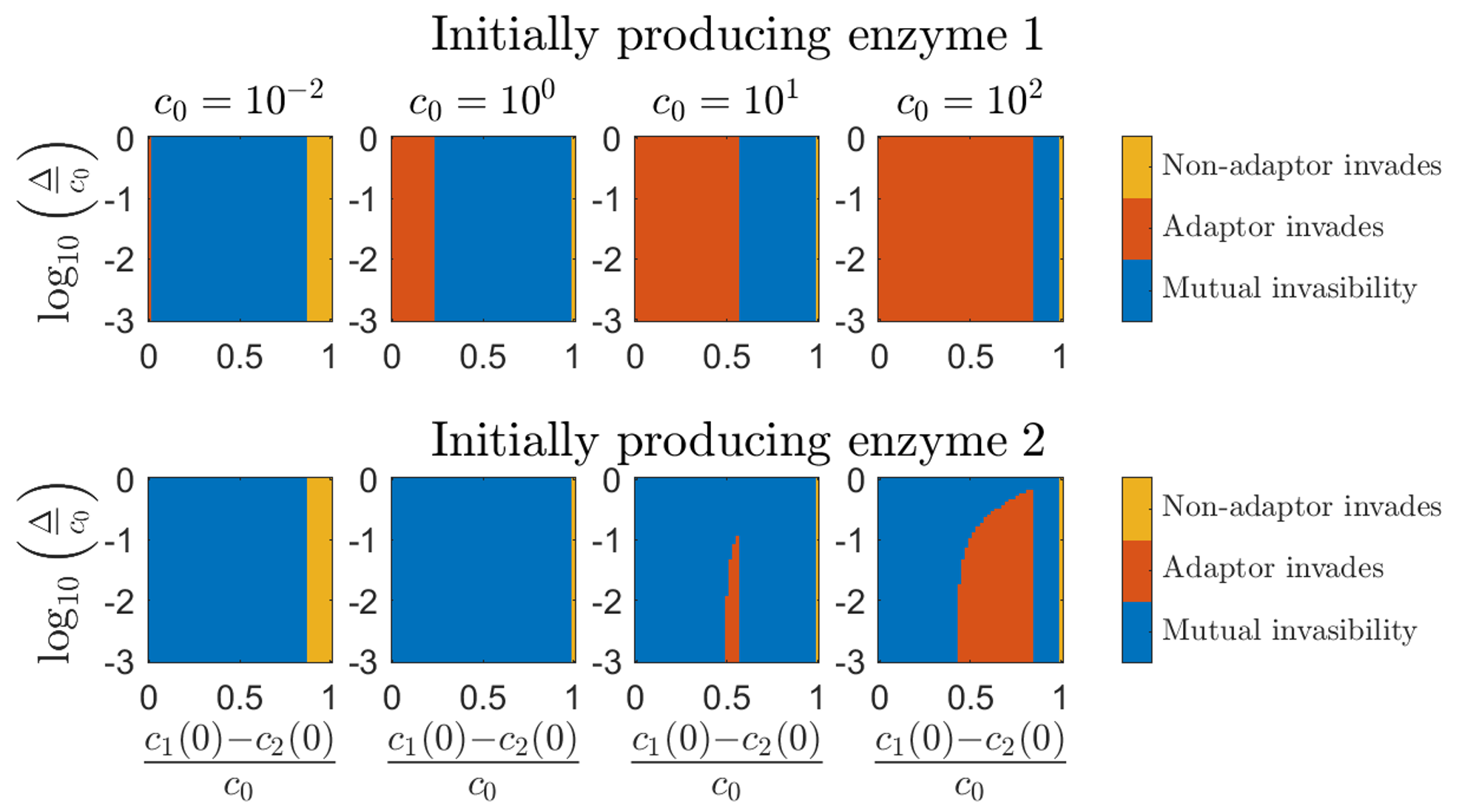
A consumer-resource modeling framework in a serial-dilution setup, where $m$ species compete for $p$ nutrients in a series of batches. At each batch, a nutrient mixture is supplied with a fixed composition $\lbrace c_i(t=0)\rbrace_{i=1}^p$ and total amount $c_0=\sum_i c_i(0)$. Similarly, a mixture of species $\lbrace\rho_\sigma(t=0)\rbrace_{\sigma=1}^m$ is added, with a fixed total amount $\rho_0=\sum_\sigma \rho_\sigma(0)$. Species grow until the depletion of nutrients, the culture is diluted, and a new batch starts, while keeping relative species populations.
Each species has a metbolic strategy, $\vec{\alpha}_ \sigma$, which is a vector of enzyme levels, while given a fixed enzyme budget $E_\sigma=\sum_i \alpha_{\sigma,i}$, leading to a metabolic trade-off. Nutrient consumption rates are given by $j_{\sigma,i}=\frac{c_i}{K+c_i}\alpha_{\sigma,i}$.
The main feature of this framework is the inclusion of species adaptation to changing nutrient levels throughout the batch, by allowing the dynamics of the metabolic strategies, given by 2:
where $\mathbb{P}_{\sigma,i}$ is an indicator function which is 1 whenever species $\sigma$ produces enzyme $i$, and 0 otherwise. The dynamics of this indicator determine the nature of the metabolic adaptation. Note that an adaptor population can only produce a single enzyme type at a time.
The framework includes a few adaptation models (i.e., different dynamical schemes for $\mathbb{P}_{\sigma,i}$; see app__simulations.m) that operate under these guidelines, and is receptible to the addition of different models that may work in this context. Note that this adaptation feature is based on the 2-nutrient case and thus is limited to $p=2$ (however, $p=1$ and $p>2$ dynmics can be simulated with no adaptation).
The dynamics are numerically solved for using MATLAB‘s built-in ode89 Runge-Kutta solver with adaptive step size. Simulations can be applied in a specific, instant manner, or by parallelly executing and collecting data from large sets of simulations, using the Split-Apply-Combine method (see below for protocol).
Script Index
Note
Here, the general structure of this repository’s Code section and the workflow are described. For a script-specific description, look at each script specifically.
odefun.m and the eventfun*.m functions (one for each adaptation model) are the most basic functions, used by ode89 as function handles to solve for the dynamics. odefun.m contains the actual dynamics, while the eventfun*.m functions are used to track events througout the dynamics.
The app__*.m scripts are the main scripts that apply the simulations, and are directly used by the user for setting parameter values and executing the simulations. app__simulations.m is used for running specific simulations (single or several), whereas the app__slurm__*.cmd files are used for implementing large simulation sets in parallel (see below).
The plot__*.m functions are used to plot the dynamics or other results (raw or collected data). Some are ‘raw’ plotters, which are used directly by the sim__*.m functions to plot the results from a single simulation, and have a name corresponding to their simulation function. Others may collect the data from large sets of simulations, either by reading raw-data files or a collected-data table (in the case of inter-batch simulations).
Split-Apply-Combine
A common approach to data-analysis, aiming to implement large simulation sets in an orderly and effective way:
Split – Produce a parameter table, such that each row contains values for all moving parameters (that vary between different simulations) for a certain simulation in the set, and a template-file to plug simulation parameters into.
This is done here by the split_runs__*.m functions.
Apply – Perform all jobs using a script that allocates resources and executes them independently in parallel. Each job uses the parameter template to plug values from a certain row in the split table, and performs a simulation. All set-simulations are directed to save raw data in the same directory.
This is done here by the app__slurm__*.cmd files.
Combine – Collect data into a table synchronously from all saved raw-data files in the simulation set. Analyze/plot various dependencies.
Collecting is done here either by using collect_data__interbatch.m in the case of inter-batch simulations, or directy by some of the plot__*.m functions in other cases.
The power of this method is in its modular nature – jobs can be applied independently; data from existing files can be collected independently at any point in time, regardless of currently running jobs.
Data and corresponding figures are automatically saved with easily identifiable, corresponding file names (including the simulation type and important parameter values), in the Data and Plots directories, respectively. Their general structure is embedded and a generic sample of data and figures is included here inside both directories.
Here are some of these figures:
1 Adaptor – Metabolic Strategy distributions (Tip: to simulate a single species, use 2 identical species)
Adaptor VS Non-Adaptor – Invasibility Character
2 Adaptors – Steady-State Populaion Bias VS Sensing Tolerances
References
Footnotes
Amir Erez, Jaime G. Lopez, Benjamin G. Weiner, Yigal Meir, and Ned S. Wingreen. Nutrient levels and trade-offs control diversity in a serial dilution ecosystem. eLife, September 2020 (Go to paper). ↩
Amir Erez, Jaime G. Lopez, Yigal Meir, and Ned S. Wingreen. Enzyme regulation and mutation in a model serial-dilution ecosystem. Physical Review E, October 2021 (Go to papar). ↩
Search Engine Evaluation and Near Duplicate Detection
University project at the course of Data Mining Technology for Business and Society concerning the building of a search engine using the Pyterrier library and the Near Duplicates Detection task.
Project Tasks
The project is divided in two main parts:
Search Engine Evaluation:
use the Pyterrier library in order to build a search engine for the ‘irds:nfcorpus/dev dataset’ and improve the search-engines performance, comparing different pipeline combination of preprocessing and weighting model, togheter with choosing in a proper way different evaluation metrics of the information retrieval task (like Normalized Discounted Cumulative Gain or Mean Recirpocal Rank) in order to understand the quality of the engine.
given several scenarios, like a company needing a search engine for the dataset of scientific paper, being able to build the proper search engine with a single specific configuration of preprocessing, weighting model and evaluation metrics, justifying the choice.
Near Duplicate Detection:
in this part of the homework, we have to find, in an approximated way, all near-duplicate documents inside a collection of documents, following the rules below.
We will consider Near-duplicates all those pair of documents that have a Jaccard similarity greater than or equal to 0.95
Each set of shingles, that represents an original document, must be sketched in a Min-Hashing sketch with a length of at most 210
The probability to have as a near-duplicate candidate a pair of documents with Jaccard=0.95 must be > 0.97
The generation process of near-duplicate pairs you implement must generate the smallest amount of both False-Negatives and False-Positives
The running time of all the LSH process must be less than 10 minutes, and motivate the choice of the hyperparameters like the row and band for the LSH.
GPU is enabled by default for Whisper/Piper/Ollama images. You can remove deploy blocks if you plan to run on the CPU. Note that this guide doesn’t cover the CUDA setup. Follow the official NVIDIA tutorials for that.
docker compose up -d
Voice Assistant PE
Follow this guide to connect your hardware. Note that if you are as lucky as me and don’t have a stable BLE device on your PC, you’ll likely get infinite Bluetooth errors on your HA instance, preventing you from establishing the initial connection with Voice Assistant. I recommend you do not waste time, and use your cell phone to connect to the HA instance on your PC and set up Voice Assistant via mobile BLE.
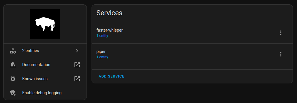
Whisper / Piper / Ollama
Whisper and Piper can be added to HA via Wyoming Protocol. As HA shares the network with your host OS, ASR / TTS services will be accessible via localhost on 10300 and 10200 ports.
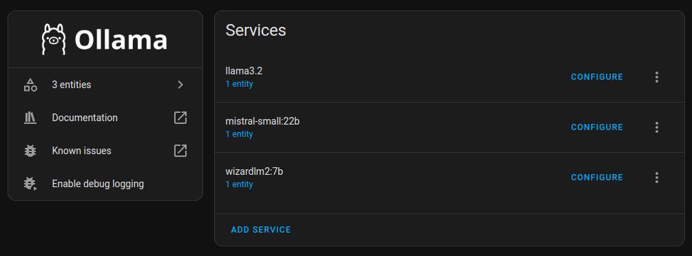
Ollama will also be accessible on http://localhost:11434. If you’ve already downloaded models locally, you’ll immediately see them as we mapped the model folder with the container.
I recommend starting with Llama 3.2. Don’t forget to tune the prompt and enable assistance:
Just so you know, if you want to add a new model, you need to add it as a separate service.
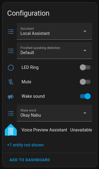
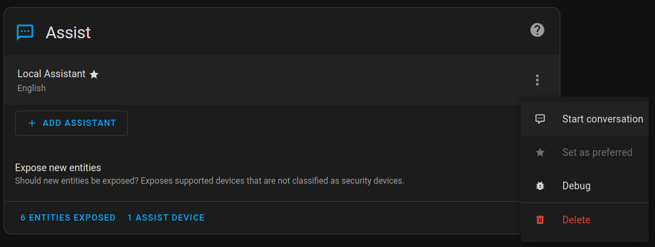
Now you can see newly added services in the Voice Assistant config:
Expose your smart home devices to voice assistant (alias will serve as a short command to access your device):
Ensure your ESPHome is linked with Voice Assist PE and connected to the newly configured virtual Voice Assistant in HA:
Test ASR / TTS and chatting capabilities via web UI:
Now you are ready to interact with your devices via Voice PE hardware and have casual conversations with Llama 3.2. Well, not really…
Known Issues
You’ll likely almost immediately face TTS failures on long responses from LLMs. There are several similar bugs raised across HA repos about this.
One workaround you can apply is patching the AudioReader timeout in the VA PE firmware code. Note that to build the firmware, you must provide your Wi-Fi credentials in secrets.yaml. You should also update the repo reference to ensure your changes are applied. Otherwise, the code will be pulled from the original dev branch.
Update external_components URL to point to your fork.
Build and flash the updated firmware:
docker run --rm -v "$(pwd)":/config -it ghcr.io/esphome/esphome run --device IP_OF_YOUR_VA_PE home-assistant-voice.yaml
Also note that changes in containers’ environment variables (e.g., new models or voices) require a complete stop. New values won’t be automatically picked up on restart.
We are team of five people we have made clone of Indeed job website in which we have done many things by using HTML,CSS and Java Script so here is what we have done
Landing_Page
This is our landing page in this page we have added functionality of searching so in which user can find company by the company name ,company location,job role etc.
If by searching data is not found then it will show no match found and if user don’t write anything in input then site give alert of “please enter something.
After that in company data whichever company you click on it will show you details of that company beside the all company data. in which user click on the apply site will give alert “please login first”.
so user have to login/signin first that option user can find in footer.
Signin_Page
This is our Sign in page in which if user have already account then they can direct sign in but if don’t have account then they can creat new account by click on signup now
Signup_Page
This is our signup page in which user can make new account if user already exist then it will give alert “user alredy exist” if user is new then they can make new account and then direct they can login.After they login they will landed to the Home page.
Home_Page
This is our home page and our Home page and Landing page are someway similer but in home page use some extra functiomality like sorting
So in this page user can sort by salary,rating,role etc.
Also in home page user can apply job and wishkist that job too
Also search company by loaction job role
Recent_Search
Whenever user search anything it will show in recent search
Company_Reviews
In Header by clicking Company reviews user landed on that page in which user find company and they can see reviews of that company
Salary_Guide
In Header by clicking Salary guide user can salary provide by many company
Message
In header by clicking on message icon use can see latest mesaage
Notification
In header by clicking Notification icon use can see latest notifications.
Profile
In header by clicking Profile icon use can see list 1) My Job 2) Signout
By clicking Signout user direct landed on landing page.
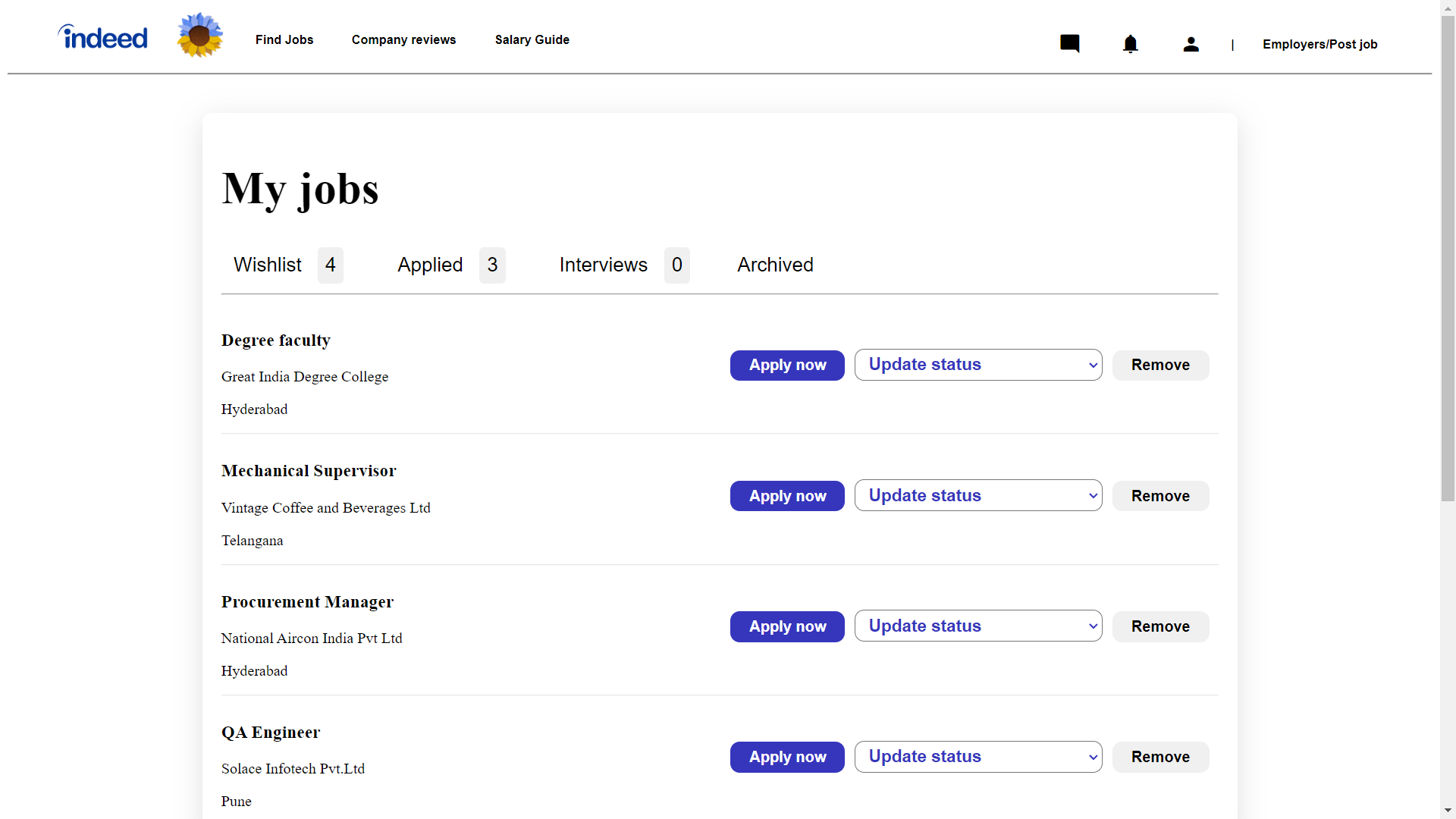
My Jobs
By clicking my jobs it will show user job that was added or wished by user
In this page we have added my functionality so in which user can remove job from wish list and applied list also they can move wished job in to applide job also vise versa


_-2.p.png)

_-2.png)